
You Can’t Differentiate a Metaphor
Conceptual vs Mathematical Spaces in Molecular Biology

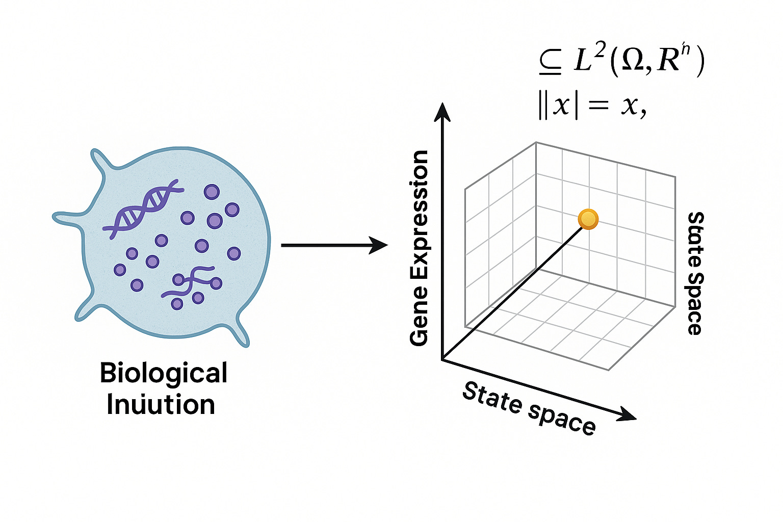
Biological intuition seduces us with language like “gene expression space” or “metabolic state space,” but these are conceptual shadows. What lives in the notebooks of molecular biologists is not yet a space in the mathematical sense. The CELL initiative demands we be precise: a space is not a metaphor, it is a structure. A state space must admit norms, inner products, convergence, and operators. Without those, it cannot support a calculus. And without a calculus, there are no gradients, no adjoints, no control.
Let us take the molecular scale as a worked example.
This article is in continuation of “Adjoints; Or It Did Not Happen”…
The Conceptual Biological Space
At the molecular level, one might say an organism exists in a “space” of transcriptional states or proteomic profiles. This is a finite-dimensional heuristic: each axis corresponds to a gene, a protein, or a metabolite, and the value on that axis is some measure of expression or abundance. In this language, the biological state of a cell at a given time is a point in this high-dimensional space.
But this picture breaks down as soon as you ask serious questions. What is the topology of this space? What is the metric? What is the algebra that defines its dynamics? The conceptual space has no answer. It is a naming scheme, not a model.
From Notion to Structure
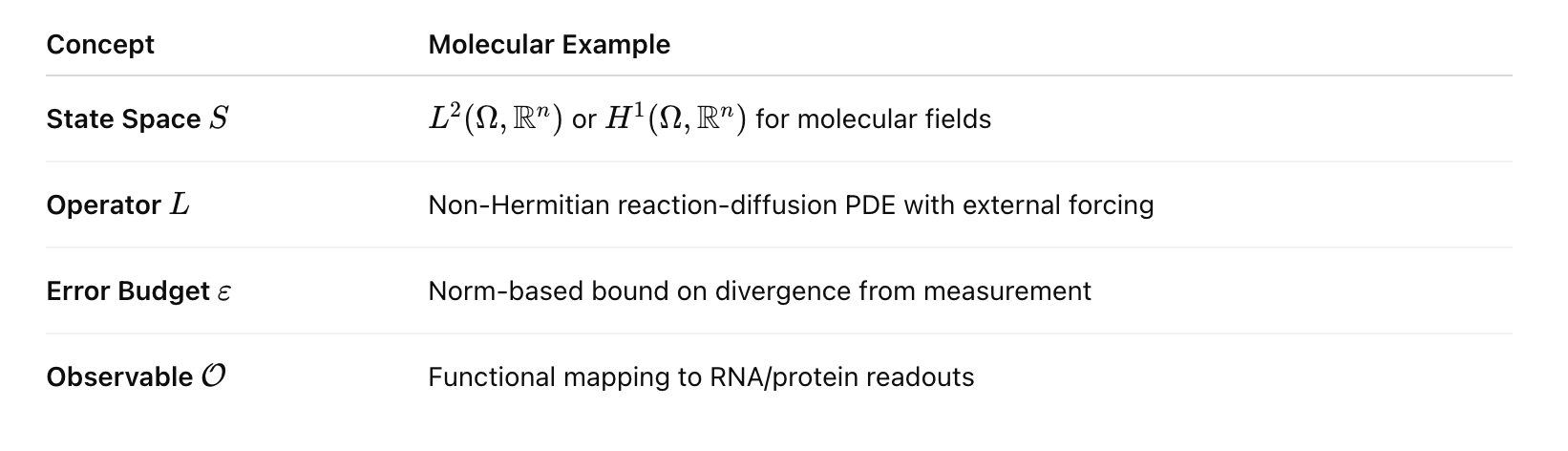
In CELL, we aspire to formalize the molecular state space as a functional space. Let S denote the state space of molecular concentrations and configurations. A minimal construction is S ⊂ L^2 (Ω, R^n), where Ω is the spatial domain (say, the cytoplasm of a cell) and each function x_i(x) in the vector-valued field represents the concentration of species i at position x.
This is not symbolic bookkeeping. The L^2(Ω) space provides a Hilbert structure with the inner product:

which induce a geometry on the state space. From here, we can define projection operators, energy functionals, and eventually, dynamics.
When spatial gradients or higher-order regularity are required, we move to Sobolev spaces H^1(Ω) or more generally H^k(Ω) for partial differential operators with boundary conditions. These spaces let us describe diffusion, gradients, and fluxes with mathematical precision.
The Operator L
In any CELL-consistent framework, dynamics are given by an operator:

The operator L encodes biophysical dynamics. At the molecular scale, a typical form is:

where Δ is the Laplace operator over Ω, D_i is a diffusion coefficient, and f_i encodes reaction kinetics (e.g., mass-action, Michaelis-Menten, Hill functions), defined over a domain Ω with appropriate boundary conditions (Dirichlet or Neumann). The operator is understood as:

where the nonlinear reaction term f_i(x) may be linearized locally for spectral analysis.
Note: the operator L is almost always non-Hermitian.
Why Biological Operators Are Non-Hermitian
This is not a curiosity. It is a necessity. Hermitian operators are self-adjoint with respect to a given inner product, and thus have real eigenvalues and orthogonal eigenfunctions. This is only compatible with systems that are closed, conservative, and time-reversible. Biology is none of these.
Strictly speaking, in infinite-dimensional functional analysis, we distinguish between symmetric, self-adjoint, and sectorial operators. Our use of “non-Hermitian” here refers broadly to operators that are not self-adjoint with respect to the L^2 inner product and therefore lack real spectra and orthogonal eigenspaces.
Biology is open, dissipative and non-equilibrium states.
Let’s unpack that.
1. Open Systems
Biological subsystems exchange energy, mass, and information with their environment. For example, nutrient uptake or drug influx is modeled via source terms or boundary inputs:

where u_i is an external control or flux. This violates conservation.
Mathematically, open systems introduce non-self-adjoint terms, breaking Hermiticity:

2. Dissipative Systems
Living systems continually lose usable energy to entropy. ATP hydrolysis, protein degradation, transcriptional noise, all involve dissipation.
Consider a linear operator:

for some decay rate γ > 0. The eigenvalues are negative reals. The semigroup e^{Lt} decays in norm. The system is contracting. Such L is dissipative and cannot be Hermitian unless γ = 0, which corresponds to unphysical, non-decaying trajectories.
3. Non-Equilibrium Systems
Steady-state in biology does not imply thermodynamic equilibrium. A cell can maintain stable concentration profiles (e.g., ion gradients across a membrane) while being far from equilibrium. These are sustained by continuous energy input.
Such systems require non-normal operators, ones whose eigenvectors are not orthogonal, and whose transient behavior can amplify perturbations even when all eigenvalues are negative. This breaks the assumptions of Hermitian linear algebra.
The Error Budget ε
No model is perfect. CELL requires every model to carry an error budget ε that explicitly bounds the deviation between model predictions and reality:

The norm must be defined by the state space. In L^2, this means squared difference in concentration fields. In practice, the error budget has multiple components:
Model error: approximation of biology by equations
Numerical error: discretization, solver tolerance
Parameter error: uncertainty in rate constants
Measurement noise: empirical bounds on experimental input
The error budget is not a disclaimer. It is a certificate. Without it, models are decorations.
The Observable O
A model that cannot return observables is not a model. It is a memo. In CELL, we demand that for each system, we specify observables O : S → R^k that represent quantities we can interrogate.
At the molecular scale, observables may include:
Fluorescence intensity from tagged proteins.
mRNA abundance from single-cell RNA-seq.
Protein concentrations from mass spectrometry.
Molecular flux across a boundary.
Each observable corresponds to a functional:

where w_i(x) is a weighting kernel reflecting the measurement modality.
Observable functionals are the hooks by which models touch the empirical world. They must be defined as part of the model spine.
Toward a CELL Spine at the Molecular Scale
At CELL we hypothesize that at each biological scale, we define:
This spine is not optional. It is the prerequisite for building models that are not merely symbolic or heuristic but carry the full weight of analysis. Only with a defined space, operator, observable, and error budget can a system admit adjoints, enable control, and integrate into a scalable architecture for biology.
CELL’s mission is to make biology legible to mathematics and actionable by design. That means retiring metaphors of “states” and “spaces” that do not survive mathematical scrutiny. The cost of rigor is high. But the cost of staying vague is higher.
Metaphors are great to help us understand the world around us, but we need equations to make biology executable.
Join us and shape the debate.
Follow us on our channel for updates here on X
Note: This article presents a working hypothesis, not a settled doctrine. We invite the community to refine, and co-build this blueprint in the collaborative spirit of open science.