When Does an Equation Become an Equation of Life?

A zebrafish embryo reveals what mathematics must preserve across genes, mechanics, and fate

Whenever I utter the words “equations of life,” people immediately assume a closed-form expression that receives a genome, a cell, or an organism and returns its future. That image confuses an equation with a closed-form solution and a formula with a scientific model. It is not what an equation is.

An equation is a formal statement about how selected quantities relate. It may express a constraint, a rate of change, a probability law, a conservation principle, an observation process, or a condition connecting two descriptions. Some equations admit analytical solutions, occasionally in closed form. Others are studied through controlled approximations, numerical solvers, stochastic simulation, or qualitative analysis of stability, thresholds, and bounds. These are not lesser substitutes for mathematics. They are different ways of extracting consequences from a formal model.

Approximations and numerical solutions must establish convergence and quantify error. Whatever the solution method, a scientific model must also be compared with evidence. Strictly speaking, an equation becomes such a model only when its variables, units, parameters, domain, initial and boundary conditions, measurements, and regime of validity have been specified.

An equation earns the name “equation of life” when it makes a precise, testable, regime-bound claim about a living process. It does not need to contain the whole organism in one line. One equation may describe gene regulation, another tissue mechanics, and another morphogen transport. When those equations participate in an explanation that crosses biological descriptions, an additional obligation appears. The consequences passed between them must also survive experiment. Each equation may succeed on its own measurements while the biological explanation fails at the handoff.

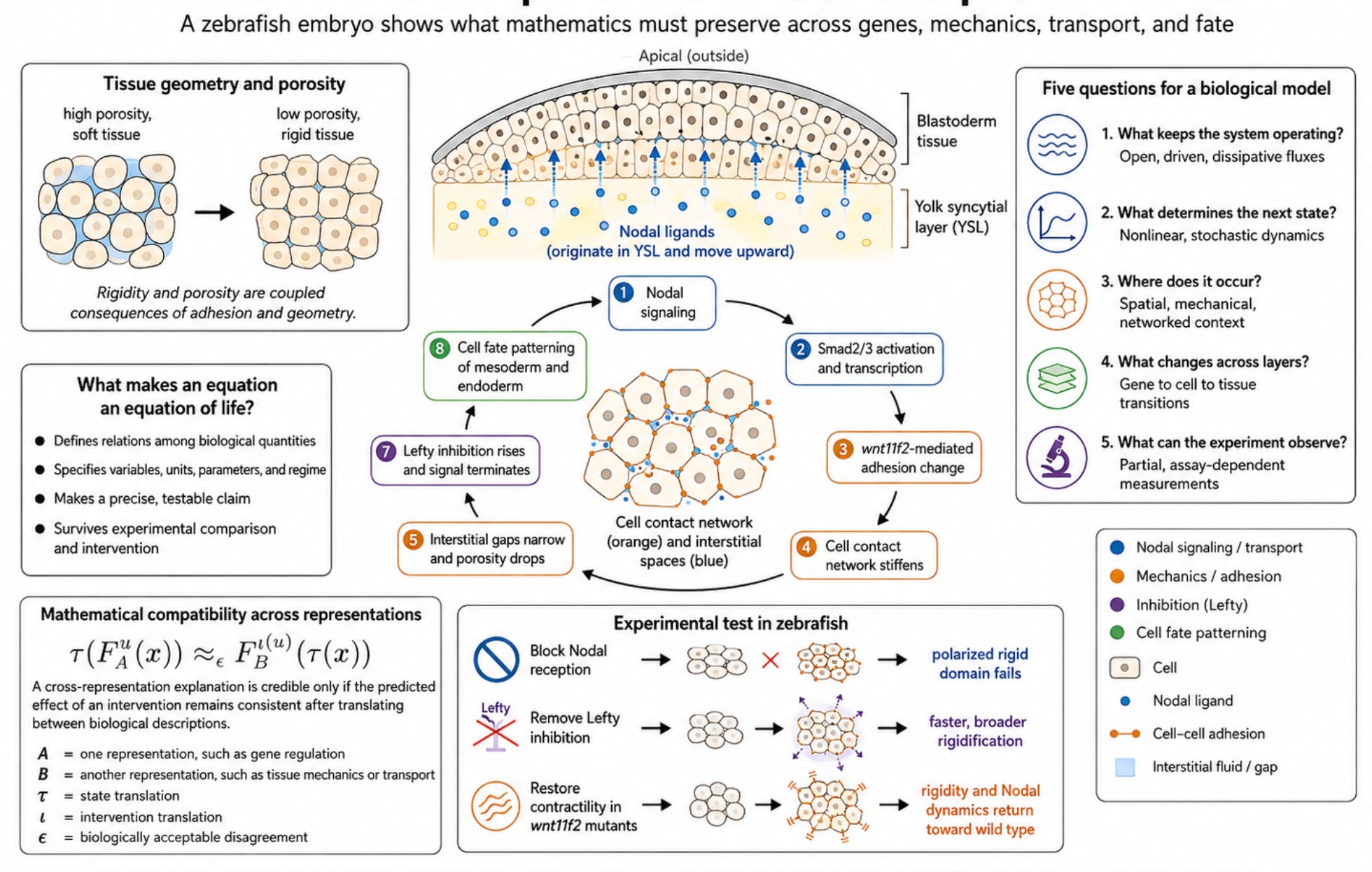
In an early zebrafish embryo that was recently published, that handoff becomes visible. A secreted signal called Nodal helps determine which cells will contribute to muscle, blood, gut, and other tissues. But Nodal does not merely move through the embryo and deliver an instruction. It changes the material through which it travels, and the changed material alters how far the signal moves and how long it lasts. Before following that loop, we need to decide what kind of system an equation in biology is being asked to describe.

Five questions organize the problem.

1. What keeps the system operating? When active, living systems are open, dissipative, driven, and resource-constrained, although some local processes admit equilibrium approximations. A metabolic model therefore foregrounds material and energetic flux.

2. What determines the next state? Biological dynamics can be nonlinear and stochastic. A description is approximately Markovian when its retained present makes the future conditionally independent of earlier history over the declared horizon. Omit relevant chromatin, lineage, protein state, or mechanical history, and the reduced description may acquire memory, although some coarse-grainings preserve Markovianity. RNA dynamics can be stochastic, while transcriptomic assays reveal only part of the process. Signalling adds feedback, thresholds, and delays.

3. Where does the process occur? Biology is spatial, compartmentalized, mechanical, and networked. Cells exchange neighbors, generate forces, reshape boundaries, and modify the routes through which signals move. Geometry and connectivity can be part of the state.

4. What changes across biological layers? Genome, epigenome, transcriptome, and proteome describe molecular layers. Metabolism describes processes, while cells, tissues, organisms, and populations describe organizational levels. Experiments represent them as sequences, count distributions, fluxes, fields, graphs, and trajectories. The relations are partial, context-dependent, and often stochastic. Feedback can run in both directions without making those relations invertible.

5. What can the experiment actually see? Biology is partially observed. Assays make some structures measurable while leaving other causes latent, and measurement can perturb the system. Sequencing exposes RNA counts while losing contacts and forces. Imaging preserves location but usually follows fewer components.

The answers to those five questions change as we move through a living system. A molecular reaction, a cell state, a tissue deformation, and an evolutionary trajectory are not the same object viewed at different magnifications. They differ in timescale, organizational level, how we measure them, and the kinds of causes we can resolve. Scale in biology therefore has several axes.

Spatial extent runs from molecular dimensions to ecosystems. Timescale runs from reaction events to evolutionary change. Organizational level runs from molecular assemblies to populations. Observational resolution and modality determine whether an experiment yields reads, images, forces, or trajectories. Causal grain distinguishes local interactions from collective behavior. These axes overlap but are not interchangeable. Moving from transcriptome to tissue is not simply zooming out. It changes what counts as a state, an interaction, and an explanation.

Nor do the layers form a clean ladder. Transcription changes the RNA available for protein synthesis. Proteins alter metabolism and mechanics. Mechanics changes transcription, while the environment changes which genomic differences matter. Across generations, individual trajectories coexist with distributions shaped by heredity, mutation, reproduction, and selection.

Nature does not contain these layers as separate machines, and it does not perform translations between them. We do. The embryo remains one coupled process. The handoff appears when one representation is asked to preserve a consequence discovered in another. The problem is testing whether that translation preserves the response we intend to predict.

The zebrafish experiment followed several such translations through one developmental event. The blastoderm contains loosely attached cells separated by interstitial fluid. Nodal ligands produced in the yolk syncytial layer enter this tissue and activate the phosphorylation of Smad2/3 in nearby cells. Smad2/3 accumulates in the nucleus and changes transcription. Cells interpret the local amplitude and duration of this signalling as positional information that helps specify mesoderm and endoderm.

But the field does not move through a passive container.

Nodal also regulates wnt11f2, which changes adhesion between cells. The study described the resulting material reorganization in two coupled ways. In the contact network, cells were represented as nodes and their contacts as bonds. A constrained cluster percolated across the tissue when connectivity and adhesion crossed the regime associated with rigidity. The average connectivity was near four contacts per cell in this experiment, but four is not a universal biological threshold. Tissues with the same average connectivity can differ in rigidity because the arrangement and geometry of their constraints also matter.

The second description concerned the spaces between cells. The investigators measured contact angles and used the Young–Dupré relation to infer a dimensionless ratio of cell-cell and cell-fluid surface tensions. As adhesion changed those angles, small fluid gaps at tricellular contacts closed. Further geometric change reduced the remaining three-dimensional porosity. Rigidity of the cellular network and collapse of the interstitial network were coupled consequences of adhesion and contact geometry. One was not simply passed into the other as a causal input.

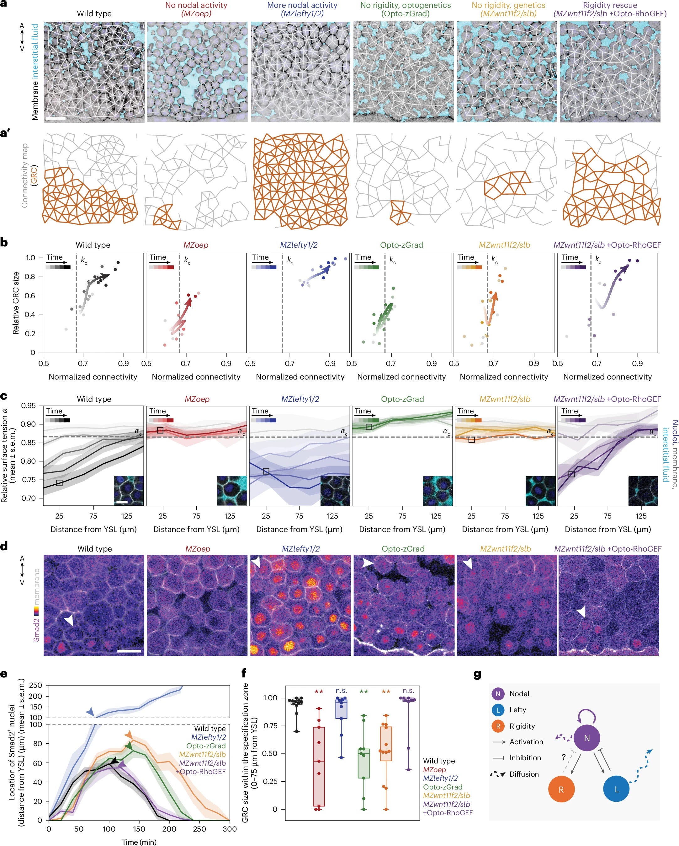
The interstitial geometry then acted back on Nodal. As extracellular routes narrowed and disconnected, the effective dispersal of the ligand changed. Nodal and Lefty could be represented as fields over space and time, with production, inhibition, and degradation entering as reaction terms. Their transport, however, was not simple diffusion through an inert medium. Receptor binding, cellular uptake, secretion, hindered movement, and signalling relay can all shape the observed range. The specific result was that tissue porosity altered Nodal’s effective diffusivity, concentrating signalling near the source and accelerating expression of Lefty, which inhibits Nodal and helps terminate the response.

Our description of the biology had now crossed several mathematical forms. Gene regulation altered adhesion. Adhesion changed a contact network and an extracellular geometry. That geometry altered effective transport. Transport changed signalling and transcription. None of these conversions was justified merely because the individual model on each side fit its own data.

The logic of such a test can be written compactly. Let F_A^u​ describe the response predicted in representation A after intervention u. Let τ translate states from representation A into representation B, while ι translates the intervention itself. Compatibility asks whether

The left side applies the intervention first and then translates the result. The right side translates the starting state and intervention first, then predicts within the second representation. Agreement is judged for a declared observable, time horizon, biological regime, and tolerance ε. That tolerance need not be small in the abstract. It must be small enough that the biological conclusion being tested does not change. If the two routes disagree beyond it, the translation has failed for that claim, even when both equations fit the measurements on which they were built.

The notation is deterministic shorthand. Neither translation must be exact, invertible, or valid everywhere. A predicted response may be a state, a trajectory, or a probability distribution. When the biology is stochastic, τ may relate distributions rather than individual states. The intervention map ι exists only for interventions preserved by the abstraction. If no counterpart exists in the second representation, that intervention lies outside the model’s valid regime. A handoff earns credibility by predicting an intervention, context, or timepoint that was not used to construct it.

The zebrafish study did not formulate τ or ι, estimate ε, or formally certify the compatibility condition. It did not need to. The notation is not a protocol for discovery. It states what a cross-representation explanation commits us to test.

The study’s perturbations supplied evidence for the proposed handoffs. Embryos unable to receive Nodal failed to form the normal polarized rigid domain. Embryos lacking Lefty inhibition rigidified more rapidly and extensively. When light-induced degradation of alpha-catenin prevented normal rigidification, nuclear Smad2 activation appeared in more distant cells and persisted longer. These interventions challenged any account in which tissue mechanics was merely a passive consequence of patterning.

The more discriminating experiment bypassed the damaged biochemical link. In wnt11f2 mutants, the normal adhesion gradient and rigidity pattern were disrupted, while Nodal signalling became broader and more persistent. The researchers then used a different light-controlled system to increase contractility. This restored the adhesion gradient, tissue rigidity, and wild-type-like spatial and temporal Nodal dynamics without repairing wnt11f2. The mechanical perturbation produced the biochemical response expected at the next handoff. The rescue did not identify one uniquely true model, but it rejected the passive-background account under the tested conditions and supported the proposed mechanochemical coupling.

The experiment does not solve the general problem. It shows what mathematical credibility across biological descriptions demands. Applied mathematics already names pieces of that problem as closure, coarse-graining, constitutive modelling, causal abstraction, and multiphysics coupling. Statistical physics contributes effective descriptions across scale. None of those formalisms, by itself, decides which biological state, measurement, intervention, or consequence matters. Biology makes the interface obligation unusually severe because its representations are often built by different experiments, carry different hidden histories, and may change while the organism develops.

None of this diminishes a model that succeeds within a declared regime. A model that predicts a mutant or guides an intervention has earned that local claim. The additional obligation begins only when the model is used to explain how a consequence in one biological description produces a consequence in another.

A mathematician could still place chemistry, mechanics, geometry, lineage, metabolism, and every measurement process inside one sufficiently large dynamical system. In principle, one formal object can contain them all. That does not remove the scientific problem. The issue is whether we can derive or learn smaller representations whose predictions remain compatible under interventions we can actually perform. Every reduction introduces a handoff, and every handoff creates a new place for the explanation to fail.

An equation of life is therefore not a definition of life or a molecular inventory. It is a regime-bound representation that makes an experimentally accountable claim about a living process. When that claim crosses into another representation, the translation must state what information is carried forward, what is discarded, which interventions it preserves, and how much disagreement is allowed. Interventional sufficiency belongs not only inside each model but at the boundary where one model supplies meaning to another.

A living system does not decompose itself into the representations through which we study it. The embryo remains whole even when our mathematics does not. If an explanation survives within each model but if the biological consequence disappears at their boundaries, was it ever an explanation of life?