
From Markers to Manifolds
A configuration space for cell fate that biologists can run and mathematicians can analyze

On a good day in the lab you get what you planned for. On a better day you get what you planned for and you understand why. To understand what we are trying to achieve at CELL, the paper I want to anchor this with is by Sáez, Blassberg, Camacho-Aguilar, Siggia, Rand, and Briscoe, “Statistically derived geometrical landscapes capture principles of decision-making dynamics during cell fate transitions.” They take the familiar Waddington picture and turn it into a working instrument for stem cell fate. Not a poster. A model that can be built from flow data, fit to timed Wnt and FGF schedules, then used to forecast new schedules and the split of fates you will actually see on day three, four, five. That is rare and valuable. It is also the right starting point for a universal configuration space for molecular biology that is reproducible, interoperable, and robust across labs and organisms.
CELL is an open consortium that brings mathematical biology, biophysics, and computational biology together around a shared mathematical core.
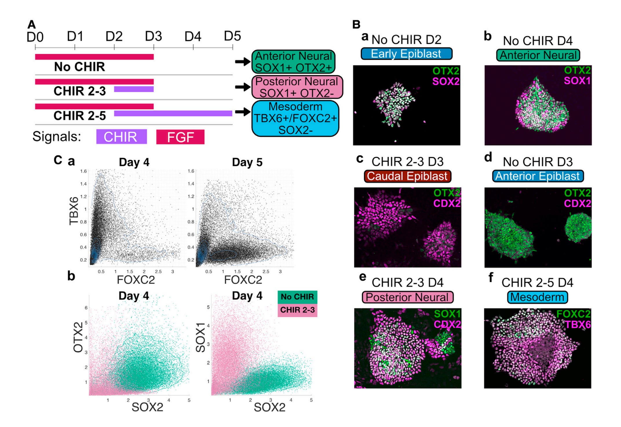
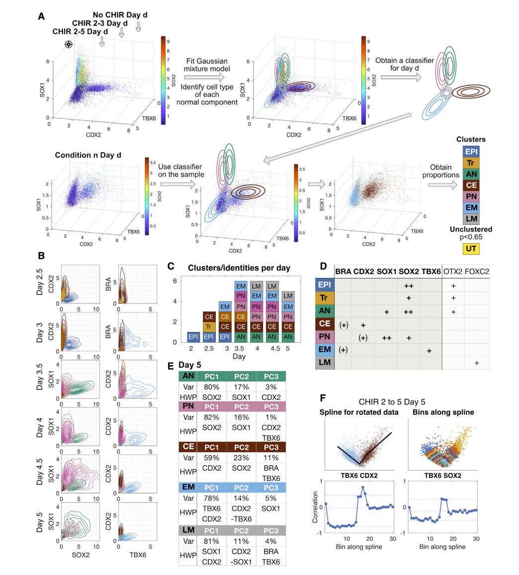
The story in their hands is practical. Mouse ESCs are walked through an epiblast-like progenitor, then pushed toward anterior neural, posterior neural, or mesoderm under controlled Wnt and FGF programs. The authors measure a small set of markers by flow and imaging, call the major states without supervision, and treat these as attractors in a low dimensional landscape. You can see the itinerary in their schematic with CHIR and FGF bands that encode when signals are on or off, and the fate identities that dominate at day five. OTX2 sits high in anterior neural. CDX2 marks caudal epiblast and posterior neural. TBX6 then FOXC2 capture early and late mesoderm. The link from markers to attractors is made concrete in their clustering analysis where mixture components line up with cell types and the sharp change in local marker correlations reveals the edges between basins. Those boundaries behave like separatrices (the boundary that divides basins of attraction), not vague gradations, which is exactly what a landscape predicts when cells pass between stable states.
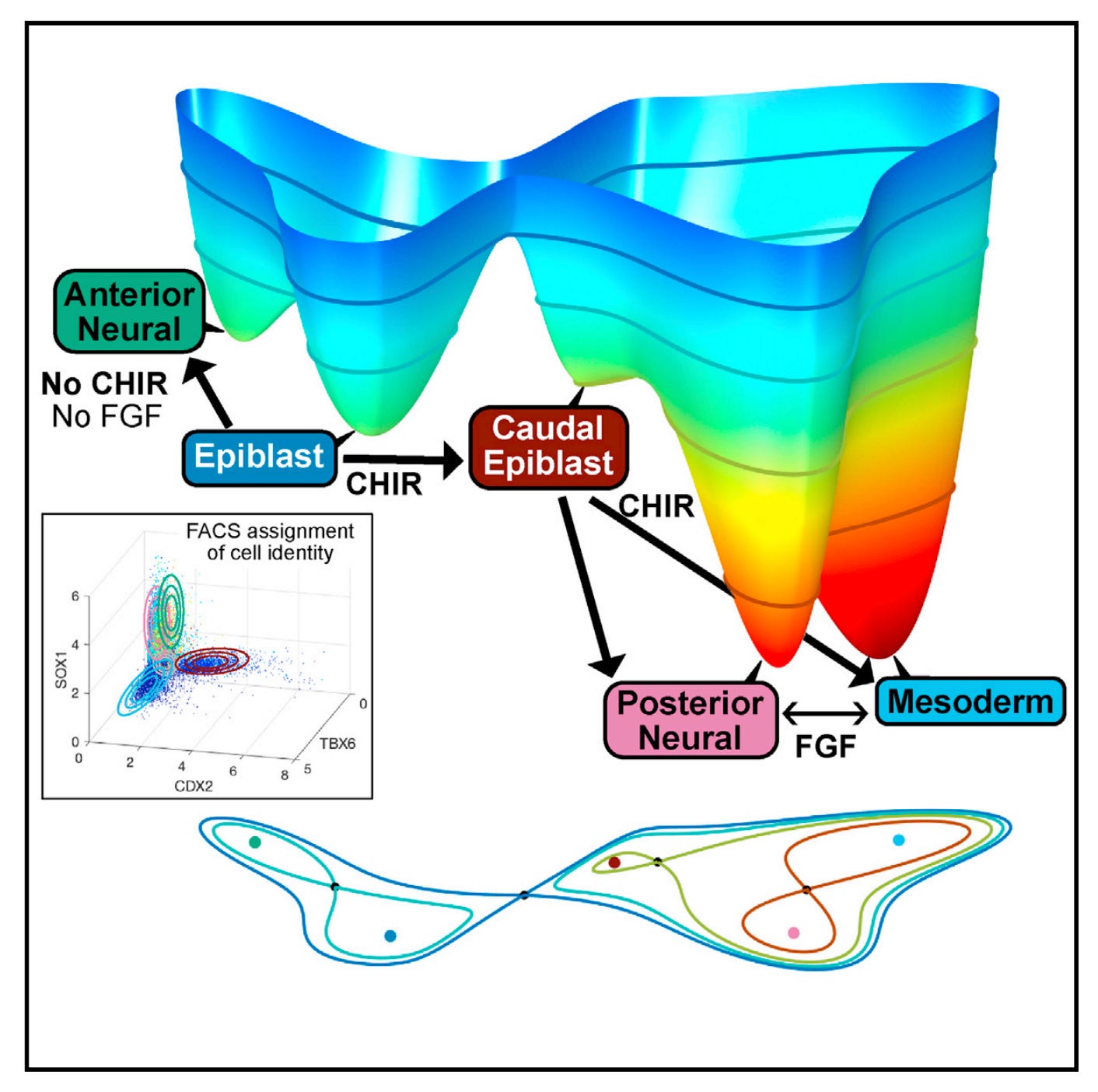
Once the states are named and counted, the geometry comes into view. Two decision designs cover the biology. In the first, the epiblast basin is lost at a threshold and the whole cohort commits together to either anterior neural or caudal epiblast. In the second, a shallow caudal epiblast basin persists and continuously feeds posterior neural or mesoderm, with the preferred exit on the unstable manifold (the direction a system leaves a saddle) flipping as Wnt and FGF tilt the terrain. Those two normal forms, a binary choice and a binary flip, are drawn explicitly with three attractors each, with saddles between them, and with signal-controlled parameters that move hills and valleys. The choice module and the flip module are stitched at the shared caudal epiblast attractor into a single five-attractor landscape. This is not a cartoon. It is the minimal geometry that fits the observed commitments and allocations, and it is exactly what catastrophe theory would have asked you to try first.
Fitting is done with summary statistics that matter at the bench. Fate proportions over time under defined schedules, not a thousand transcript features. The authors use simulation based inference to learn the map from signals to landscape shape and to calibrate the noise that drives escapes from shallow basins. The head-to-head between predicted and measured fate fractions under training and withheld schedules covers the usual cases and the hard ones. Late Wnt plus FGF challenges. Single and double pulses near a threshold. Dose sweeps after the progenitor stage. The first fit underestimates persistence in caudal epiblast. They fix it by adding a short Wnt memory that persists only when exposure crosses a threshold and by learning a sigmoidal CHIR dose response. That one change corrects allocation after pulses and improves dose prediction, which is what you want if the model is going to plan schedules rather than re-explain what you already did.
Why this works for biologists is simple. You do not need a full wiring diagram to steer fate. You need a faithful terrain in which the identities you care about are stable basins, the transition ridges are visible, and the signals you can apply tilt the surface in ways you can predict. Once that is in place you can answer practical questions. When does anterior neural become truly committed so that a late Wnt push will not change it. How much Wnt memory is accumulating after a pulse. Where is the saddle that will end a safe progenitor basin if you overshoot. The late Wnt challenge shows OTX2 staying high when Wnt plus FGF are added after commitment, which tells you the saddle between anterior neural and caudal epiblast remained in place and the valley was deep. Retinoic acid and FGF inhibition destabilize caudal epiblast and expand posterior neural at the expense of the intermediate, without erasing mesoderm already produced. These are clean, testable consequences of where saddles and shallow basins sit.
Here is why this matters beyond one lineage. A configuration space that names its states, declares its operator, and fixes an error budget earns constraints that travel. The chart is a hypothesis tied to the marker panel. If a transient progenitor is missed, basins will be wrong. We treat the chart as revisable: re-estimate with new markers, test on held-out schedules, and use a quick topology check to ensure the number of basins in the data matches the number in the model before fitting anything else. Attractors become testable identities. Separatrices become measurable boundaries in markers. Bifurcation points become real thresholds in schedules. Shallow basins leak at a calibrated rate. Wnt memory persists only after a threshold exposure. Those facts become priors. They shrink search, stabilize learning, and improve extrapolation the way geometric and physical priors accelerated protein structure prediction (a la AlphaFold).
How are these priors helpful for computational biology downstream?
Train a model to map schedules to fate fractions, but do not let it invent a third basin when the data support two.
Do not allow a late Wnt push to revert committed anterior neural when the saddle held in both data and landscape.
Penalize solutions that violate conservation or create negative populations.
Bias exploration toward schedules parked near saddles, where information lives. All of this follows once the configuration space is explicit.
Scope. This landscape is the right instrument when decisions are gradient-like and signal-driven. Some systems need other operators. Oscillators such as segmentation clocks and cell cycles need a phase and amplitude or limit-cycle module rather than a pure potential flow. Strong neighbor coupling such as Notch–Delta makes the terrain depend on local cell states, which we handle by coupling many charts through interaction kernels or fields. In noise-dominated regimes, discreteness and bursty transcription call for a Chemical Master Equation branch alongside the chart. The configuration space is built to host these operator classes side by side in one place. This article focuses on the gradient case because the data warrant it; follow-ups will lay out the oscillatory, coupled, and CME variants and how they compose. In practice these operator classes compose. A lineage can begin with a gradient decision, pass through a limit-cycle clock, and then branch again under CME-dominated noise.
Now make it shared. The contract is small by design, but it is still a contract. Flow gating, normalization, and schedule encoding vary across labs. We absorb that by shipping containerized pipelines, a minimal data schema for time-courses and schedules, and a short validation kit; modules are accepted only if they reproduce the shared schedules within their declared error budget. Keep the instrument as is, then wrap it so any lab can reuse it without translation fights: state space says what exists and where it lives, operator says what moves and how, error budget says how precise the story needs to be. Make that explicit and one lineage becomes a module that drops into a configuration space other systems can inhabit.
For biologists, the state space is two pieces. A low dimensional chart where each cell has a latent coordinate and a discrete fate label. A set of inputs you control in time, here Wnt and FGF. If you plan to move to tissues later, promote the inputs to fields in space and time. The operator moves cells downhill on that chart, updates the label when a ridge is crossed, and keeps a short memory for any input that leaves a footprint after a threshold exposure. The error budget fixes the tolerance you grant when predicted and observed fate fractions are compared and the level of process noise that reproduces leakage from shallow basins and the width of within-fate spreads. Publish the observation map so fate calling and boundary checks are identical across labs. With that wrapper in place, anyone can rerun the same schedules, score the same withheld designs, and see the same forecast intervals.
To make this runnable inside CELL, treat this fitted landscape as a self-contained module. Publish the small chart with its attractors and saddles, the fate-calling recipe and boundary check, the input programs you used in plates, and the short Wnt memory the pulses required. When you move to tissues, promote the inputs to fields in space and time and keep the chart intact. Fix an error budget once so forecasts carry the same intervals across labs. That is enough for other groups to replay your schedules, compare results, and compose your module with theirs.
Let me raise the ceiling and move towards mathematical biology and biophysics without losing the lab thread. The landscape behaves as a gradient system on a small manifold. Attractors are fixed points of a potential. Saddles carry one dimensional unstable manifolds that align with the exit paths you already measured. A binary choice is the loss of a progenitor minimum at a signal threshold. A binary flip is a rotation of the unstable manifold at a saddle so the preferred exit changes while the progenitor remains. Noise is not a nuisance. It sets escape rates and spreads and is calibrated to the constant leakage from a shallow caudal epiblast basin in long Wnt. The short Wnt memory is the knob that makes pulse allocations match. All of those elements are legible in the figures. The geometry you analyze is exactly what the bench probes.
Two short lines make the biophysics explicit.

z is the latent location on the fitted chart. V is the terrain, valleys are fates and ridges are boundaries, so the negative gradient carries cells toward attractors. The map from inputs and short memory to terrain shape captures how schedules tilt or reshape hills and valleys. The noise term sets leakage and spread and is tuned to match data.

c is an input field. Diffusion spreads it, decay or uptake remove it, dosing adds it. In a plate this collapses to a uniform time course. In tissues or patterned platforms it lets you place gradients and pulses where thresholds are crossed, not where the device decides.
Constraints should live inside the object, not be bolted on later. Reaction submodules respect stoichiometry and positivity. Transport conserves total mass. Cycle affinities are feasible. Information flow through the observation map does not exceed what the measured pathway can carry. Topology can police the basics before any fit. A quick persistent-homology (a way to count robust clusters or loops in high-D data) check on marker embeddings tells you how many basins the data truly support. These guardrails make forecasts stable and make models travel across datasets.
What this buys the community is a library rather than a stack of bespoke stories. Containerize the decision module you just built. Choice then flip, stitched at caudal epiblast, with the signal map and the short Wnt memory included. Ship the clustering recipe and a handful of standardized validation schedules that locate commitment points and allocation flips. Another lab can download that object and run it as is. A third lab can publish a bacterial two-component switch with the same contract. A fourth can publish a Hog1 arrest decision in yeast. Each module carries the same state space, the same operator, the same error budget. The geometry is the common language. The antibodies are not.
Downstream, these constraints become loss terms, admissibility checks, and active learning rules. They narrow the hypothesis space, reduce overfitting, and guide the next experiment toward saddles where it is most informative. That is how you turn one clear instrument into a library other models can learn from, including data-driven models that benefit from hard priors rather than drifting toward pretty but fragile fits.
We are back where we started, only stronger. On a good day you get what you planned for. On a better day you get what you planned for and you understand why. The Sáez team gave us a working instrument that does both. Our job is to preserve that instrument and give it a frame that lets anyone else pick it up, use it, and extend it. That frame is the universal configuration space. It is a small contract. It is a set of published schedules and forecasts. It is a few constraints that reflect the physics your cells already obey. It is also the way we turn one clear lineage into a common platform for molecular biology across organisms and labs.
Roadmap for the hard parts
This article is not written to declare answers. CELL exists to make the hard parts small, runnable, and shared. Each item below is a workstream that a member lab or fellow can pick up, publish as a module with a declared state space, operator, and error budget, and then submit to replay by another lab. The score is not rhetoric. The score is whether a module reproduces pre-registered schedules within its ε and publishes code to replay forecasts.
The point is to turn critiques into experiments that wroks. Where biology needs a different operator, we should build it and test composition on the same schedules. Where the chart might be wrong, we should revise it with new markers and re-score before refitting the terrain. Where pipelines drift, we should containerize them and require raw-to-fate reproducibility. This is rigorous work by design.
Universality and operator classes: We will not claim one operator fits all biology. CELL will host working groups to build a small set of operator classes that recur in practice, starting with gradient decisions, limit cycles, neighbor-coupled charts, and CME branches. Member labs publish modules side by side, then try simple compositions and score them on shared schedules.
Neighbor coupling and morphogenesis: For systems where the terrain depends on neighbors, we will run micro-pattern and organoid challenges that couple many charts through interaction kernels or fields. The goal is a minimal, reusable coupling module that recovers known patterns and survives cross-lab replay.
Oscillations and clocks: For segmentation clocks and cell cycles, we will support a limit-cycle module with phase and amplitude, then test its composition with a gradient decision upstream and downstream. Period, phase reset, and entrainment will be scored on pre-registered protocols.
Noise and discreteness: For bursty regimes, we will attach CME branches to the same state space. Single-molecule or low-copy assays will set the noise scale. Labs will show when CME improves fit or forecast at a fixed error budget.
The chart is a hypothesis: Marker sets are incomplete. We will treat the chart as revisable. Labs will run a small marker-ablation study, re-estimate the chart, and re-score on held-out schedules before any refit of the terrain.
Identifiability at fixed ε: Each module will ship a one-page identifiability table at its declared error budget. Posteriors, profile likelihoods, and sensitivities will tell us which knobs are tight, sloppy, or non-identifiable from the assays we ask people to run.
Observation pipeline and preprocessing: Gating and normalization drift across labs. We will ship containerized pipelines with unit tests and require raw-to-fate reproducibility. A simple border test based on local marker-correlation change will be part of acceptance.
Embedding validity: Before fitting anything, labs will run a quick topology check on their marker cloud to count basins, and a fold test to ensure local neighborhoods stay local on the chart. If counts disagree, expand the marker panel or add a transitional class, then re-score on the same withheld schedules.
Error budget selection: We will fix ε from replicate variance, calibration error, and readout noise, independent of the fit. The same ε will be used to score pre-registered forecasts so intervals mean what they say.
Cost of the contract: Standards are work. CELL will keep the contract small: a minimal data schema for time-courses and schedules, a short validation kit, and acceptance based on reproducing shared schedules within ε. All accepted modules publish code to replay forecasts.
Cross-lab replay: Every accepted module will be replayed by at least one external lab on its own instruments. Schedules, scoring, and ε are identical. Results and provenance will be public.
Pre-registered predictions: Each challenge will include a small set of schedules posted in advance. Labs will publish forecasts and intervals before data collection, then log hits and misses. Misses feed back into revised charts or operator choices.
Formalism without frictions: Equations will live in a short operator registry. Regularity and composition assumptions will be stated once. Articles keep biology first and link to the registry for readers who want the math.
Failure modes and red flags: We will maintain a public ledger of common failures and the guardrail that catches each. Missing transient states, miscalled borders, batch drift in signals, overconfident ε, and schedule mismatches will have simple tests attached.
Time horizon: Physics took a century. Biology will take time. CELL’s job is to organize the questions, make the tests small and public, and let member labs and fellows turn critiques into the next round of shared modules.
The effort at CELL is to turn many separate efforts into one living configuration space with shared frameworks and tests. We are not here to settle biology. We are here to make it possible for labs to build, reuse, and challenge each other’s models in the same place.